Using MAJIQ HET (ENCODE RBP knockdowns)
We have created a small example dataset from a few select genes/samples from ENCODE in order to demonstrate how to use MAJIQ. First, download the example dataset files:
[1]:
# create temporary working directory for this notebook
from tempfile import TemporaryDirectory
tempdir = TemporaryDirectory()
%cd $tempdir.name
# download archive with example data
!curl -LO http://majiq.biociphers.org/data/majiq_het_vignette.zip
# unzip and show what files are in the archive
!unzip -qn majiq_het_vignette.zip
/tmp/tmpucqll51w
  % Total    % Received % Xferd  Average Speed   Time    Time     Time  Current
                                 Dload  Upload   Total   Spent    Left  Speed
100   240  100   240    0     0  13331      0 --:--:-- --:--:-- --:--:-- 14117
100 52.6M  100 52.6M    0     0  19.8M      0  0:00:02  0:00:02 --:--:-- 18.7M
[2]:
ls
bam/            gff3/    majiq_het_vignette.zip  settings.ini
build-info.tsv  images/  output/                 vignette.ipynb
What are our inputs?
We selected RNA-seq experiments corresponding to SRSF4 knockdown (by CRISPR) vs no-target controls in K562 and HepG2 cells from ENCODE:
cell_line |
knockdown |
encode_accession |
prefix |
|---|---|---|---|
HepG2 |
SRSF4 |
ENCSR471INA |
ENCSR471INA.rep1 |
HepG2 |
SRSF4 |
ENCSR471INA |
ENCSR471INA.rep2 |
HepG2 |
SRSF4 |
ENCSR929JKA |
ENCSR929JKA.rep1 |
HepG2 |
SRSF4 |
ENCSR929JKA |
ENCSR929JKA.rep2 |
HepG2 |
notarget |
ENCSR105NML |
ENCSR105NML.rep1 |
HepG2 |
notarget |
ENCSR194SPW |
ENCSR194SPW.rep2 |
HepG2 |
notarget |
ENCSR805TIZ |
ENCSR805TIZ.rep1 |
HepG2 |
notarget |
ENCSR805TIZ |
ENCSR805TIZ.rep2 |
HepG2 |
notarget |
ENCSR853AOV |
ENCSR853AOV.rep1 |
HepG2 |
notarget |
ENCSR853AOV |
ENCSR853AOV.rep2 |
K562 |
SRSF4 |
ENCSR905NIK |
ENCSR905NIK.rep1 |
K562 |
SRSF4 |
ENCSR905NIK |
ENCSR905NIK.rep2 |
K562 |
SRSF4 |
ENCSR939BTN |
ENCSR939BTN.rep1 |
K562 |
SRSF4 |
ENCSR939BTN |
ENCSR939BTN.rep2 |
K562 |
notarget |
ENCSR005JBU |
ENCSR005JBU.rep2 |
K562 |
notarget |
ENCSR015KGT |
ENCSR015KGT.rep1 |
K562 |
notarget |
ENCSR163JUC |
ENCSR163JUC.rep2 |
K562 |
notarget |
ENCSR772DUM |
ENCSR772DUM.rep1 |
K562 |
notarget |
ENCSR772DUM |
ENCSR772DUM.rep2 |
We downloaded fastqs for these samples, aligned them to GRCh38, and took the subset of aligned reads corresponding to the following genes/genomic regions:
seqid |
start |
end |
gene_name |
gene_id |
|
|---|---|---|---|---|---|
0 |
1 |
29147743 |
29181987 |
SRSF4 |
gene:ENSG00000116350 |
1 |
1 |
32179686 |
32198285 |
TXLNA |
gene:ENSG00000084652 |
2 |
17 |
43170481 |
43211689 |
NBR1 |
gene:ENSG00000188554 |
3 |
19 |
5158495 |
5340803 |
PTPRS |
gene:ENSG00000105426 |
4 |
21 |
42879644 |
42913304 |
NDUFV3 |
gene:ENSG00000160194 |
5 |
3 |
152243828 |
152465780 |
MBNL1 |
gene:ENSG00000152601 |
6 |
7 |
43608456 |
43729717 |
COA1 |
gene:ENSG00000106603 |
7 |
8 |
101177878 |
101206193 |
ZNF706 |
gene:ENSG00000120963 |
The resulting BAMs are located in the folder bam/:
[3]:
ls bam/*.bam
bam/ENCSR005JBU.rep2.subset.bam  bam/ENCSR805TIZ.rep2.subset.bam
bam/ENCSR015KGT.rep1.subset.bam  bam/ENCSR853AOV.rep1.subset.bam
bam/ENCSR105NML.rep1.subset.bam  bam/ENCSR853AOV.rep2.subset.bam
bam/ENCSR163JUC.rep2.subset.bam  bam/ENCSR905NIK.rep1.subset.bam
bam/ENCSR194SPW.rep2.subset.bam  bam/ENCSR905NIK.rep2.subset.bam
bam/ENCSR471INA.rep1.subset.bam  bam/ENCSR929JKA.rep1.subset.bam
bam/ENCSR471INA.rep2.subset.bam  bam/ENCSR929JKA.rep2.subset.bam
bam/ENCSR772DUM.rep1.subset.bam  bam/ENCSR939BTN.rep1.subset.bam
bam/ENCSR772DUM.rep2.subset.bam  bam/ENCSR939BTN.rep2.subset.bam
bam/ENCSR805TIZ.rep1.subset.bam
Running the MAJIQ Builder
To analyze RNA splicing in these experiments we need to run the MAJIQ builder to:
define splicegraphs of annotated junctions and retained introns between gene exons,
obtain coverage over the splicegraph’s LSVs for each experiment.
The resulting coverage files can be used for quantification, and the splicegraph database can be used for downstream analysis and visualization.
In order for an LSV to have coverage generated for it in these output files, MAJIQ requires at least one of its junctions or retained introns to have sufficient evidence for it in its input experiments.
An individual experiment provides supporting evidence for a junction when it passes junction filters: --minpos and either --minreads (annotated junctions) or --min-denovo (de novo junctions). For retained introns, when it passes intron filters: --irnbins and --min-intronic-cov. See majiq build --help for details on these parameters.
Support for a junction or retained intron from an individual experiment by itself is not necessarily enough. MAJIQ partitions the set of input experiments into independent build groups. A junction or retained intron is passed (considered to have enough evidence) when at least --min-experiments experiments from the same build group pass per-experiment filters in at least one build group.
The MAJIQ builder uses a configuration file to specify where the input experiments are located and how they are partitioned into build groups. Global information about experiments are specified in an [info] section:
[info]
# species/reference name for UCSC links by VOILA
genome=GRCh38
# relative or absolute path to directories (comma-separated) with bam files
bamdirs=bam/
# these ENCODE experiments are all reverse stranded
strandness=reverse
The build groups and experiments which belong to them are specified in an [experiments] section. Build groups are keys with values listing experiment names (prefixes to BAM files excluding the .bam extension) separated by commas. If we wanted to focus only on junctions and retained introns found in all experiments for a single cell-type/knockdown, we could organize this section like (setting --min-experiments to reflect how many experiments are necessary to pass):
[experiments]
HepG2_NT=ENCSR805TIZ.rep1.subset,ENCSR805TIZ.rep2.subset,ENCSR853AOV.rep1.subset,ENCSR853AOV.rep2.subset,ENCSR105NML.rep1.subset,ENCSR194SPW.rep2.subset
HepG2_SRSF4=ENCSR929JKA.rep1.subset,ENCSR929JKA.rep2.subset,ENCSR471INA.rep1.subset,ENCSR471INA.rep2.subset
K562_NT=ENCSR005JBU.rep2.subset,ENCSR772DUM.rep1.subset,ENCSR772DUM.rep2.subset,ENCSR015KGT.rep1.subset,ENCSR163JUC.rep2.subset
K562_SRSF4=ENCSR939BTN.rep1.subset,ENCSR939BTN.rep2.subset,ENCSR905NIK.rep1.subset,ENCSR905NIK.rep2.subset
If any experiment is sufficient, we can instead have a build group for each experiment:
[experiments]
ENCSR805TIZ.rep1.subset=ENCSR805TIZ.rep1.subset
ENCSR805TIZ.rep2.subset=ENCSR805TIZ.rep2.subset
# {... all of the other experiments ...}
ENCSR905NIK.rep1.subset=ENCSR905NIK.rep1.subset
ENCSR905NIK.rep2.subset=ENCSR905NIK.rep2.subset
Equivalently, we could set --min-experiments to 1.
Another reasonable possibility would be to group by accessions, which would result in the configuration in settings.ini.
For this analysis, we are interested in considering heterogeneity between individual experiments, so we’ll use settings.ini, but with--min-experiments set to 1. We specify these flags to the builder using -c settings.ini --min-experiments 1.
In addition to these input experiments/configuration file, MAJIQ requires a GFF3 describing annotated transcripts. The subset of Ensembl GRCh38 v94 annotations corresponding to our selected genes can be found at gff3/ensembl.Homo_sapiens.GRCh38.94.subset.gff3.gz. This is passed to the builder directly as a positional argument.
Finally, we must specify the builder’s output directory using a required flag. To save its output to output/build, this would be -o output/build.
Put together, we run the builder as follows:
[4]:
%%bash
majiq build \
    -o output/build \
    -c settings.ini \
    gff3/ensembl.Homo_sapiens.GRCh38.94.subset.gff3.gz \
    --min-experiments 1 \
    2> /dev/null
This produces output files:
splicegraph.sql(splicegraph database for use with VOILA)majiq.log(logging output from majiq build){experiment}.sj(intermediate files that can be used instead of bams for future runs of majiq build){experiment}.majiq(inputs for majiq quantifiers)
[5]:
ls output/build
ENCSR005JBU.rep2.subset.majiq  ENCSR805TIZ.rep2.subset.majiq
ENCSR005JBU.rep2.subset.sj     ENCSR805TIZ.rep2.subset.sj
ENCSR015KGT.rep1.subset.majiq  ENCSR853AOV.rep1.subset.majiq
ENCSR015KGT.rep1.subset.sj     ENCSR853AOV.rep1.subset.sj
ENCSR105NML.rep1.subset.majiq  ENCSR853AOV.rep2.subset.majiq
ENCSR105NML.rep1.subset.sj     ENCSR853AOV.rep2.subset.sj
ENCSR163JUC.rep2.subset.majiq  ENCSR905NIK.rep1.subset.majiq
ENCSR163JUC.rep2.subset.sj     ENCSR905NIK.rep1.subset.sj
ENCSR194SPW.rep2.subset.majiq  ENCSR905NIK.rep2.subset.majiq
ENCSR194SPW.rep2.subset.sj     ENCSR905NIK.rep2.subset.sj
ENCSR471INA.rep1.subset.majiq  ENCSR929JKA.rep1.subset.majiq
ENCSR471INA.rep1.subset.sj     ENCSR929JKA.rep1.subset.sj
ENCSR471INA.rep2.subset.majiq  ENCSR929JKA.rep2.subset.majiq
ENCSR471INA.rep2.subset.sj     ENCSR929JKA.rep2.subset.sj
ENCSR772DUM.rep1.subset.majiq  ENCSR939BTN.rep1.subset.majiq
ENCSR772DUM.rep1.subset.sj     ENCSR939BTN.rep1.subset.sj
ENCSR772DUM.rep2.subset.majiq  ENCSR939BTN.rep2.subset.majiq
ENCSR772DUM.rep2.subset.sj     ENCSR939BTN.rep2.subset.sj
ENCSR805TIZ.rep1.subset.majiq  majiq.log
ENCSR805TIZ.rep1.subset.sj     splicegraph.sql
Running the MAJIQ quantifiers
We quantify and test for differences in PSI between independent samples from the different cell lines/knockdowns using majiq heterogen.
[6]:
%%bash
majiq heterogen -o output/heterogen/ -n K562_SRSF4KD HepG2_SRSF4KD \
    -grp1 output/build/ENCSR{939BTN,905NIK}*.majiq \
    -grp2 output/build/ENCSR{929JKA,471INA}*.majiq \
    2> /dev/null
[7]:
%%bash
majiq heterogen -o output/heterogen/ -n K562_SRSF4KD K562_NT \
    -grp1 output/build/ENCSR{939BTN,905NIK}*.majiq \
    -grp2 output/build/ENCSR{005JBU,772DUM,015KGT,163JUC}*.majiq \
    2> /dev/null
[8]:
%%bash
majiq heterogen -o output/heterogen/ -n K562_SRSF4KD HepG2_NT \
    -grp1 output/build/ENCSR{939BTN,905NIK}*.majiq \
    -grp2 output/build/ENCSR{805TIZ,853AOV,105NML,194SPW}*.majiq \
    2> /dev/null
[9]:
%%bash
majiq heterogen -o output/heterogen/ -n HepG2_SRSF4KD K562_NT \
    -grp1 output/build/ENCSR{929JKA,471INA}*.majiq \
    -grp2 output/build/ENCSR{005JBU,772DUM,015KGT,163JUC}*.majiq \
    2> /dev/null
[10]:
%%bash
majiq heterogen -o output/heterogen/ -n HepG2_SRSF4KD HepG2_NT \
    -grp1 output/build/ENCSR{929JKA,471INA}*.majiq \
    -grp2 output/build/ENCSR{805TIZ,853AOV,105NML,194SPW}*.majiq \
    2> /dev/null
[11]:
%%bash
majiq heterogen -o output/heterogen/ -n K562_NT HepG2_NT \
    -grp1 output/build/ENCSR{005JBU,772DUM,015KGT,163JUC}*.majiq \
    -grp2 output/build/ENCSR{805TIZ,853AOV,105NML,194SPW}*.majiq \
    2> /dev/null
These commands produce output to the directory specified (-o output/heterogen):
[12]:
ls output/heterogen
HepG2_SRSF4KD-HepG2_NT.het.voila  K562_SRSF4KD-HepG2_NT.het.voila
HepG2_SRSF4KD-K562_NT.het.voila   K562_SRSF4KD-HepG2_SRSF4KD.het.voila
het_majiq.log                     K562_SRSF4KD-K562_NT.het.voila
K562_NT-HepG2_NT.het.voila
These commands do the heavy lifting of inference, sampling, and testing. However, we need to use VOILA with the splicegraph database to generate human-readable outputs, as described in the next section.
Running VOILA
VOILA has three modes for looking at the output of our quantifiers:
voila tsv: generate TSVs with quantified LSVs and associated statisticsvoila modulize: generate TSVs which differentiate each specific type of splicing variationvoila view: run web service for interactively visualizing quantifications, statistics and their relationship to genes’ splicegraphs.
Generating TSV output
We can generate a TSV combining the LSVs quantified in all 6 pairs of comparisons. We:
specify the splicegraph
output/build/splicegraph.sqland voila filesoutput/heterogen/*.het.voilaas positional arguments,specify the path for our output TSV by the argument
-f output/voila_tsv/all-pairs-het.tsv,have VOILA save all quantified LSVs, not only with those called as changing using
--show-all(alternatively, runvoila view --helpto set thresholds for changing events).
This leads to the following command:
[13]:
ls output/heterogen/tmp5sw2q083/
ls: cannot access 'output/heterogen/tmp5sw2q083/': No such file or directory
[14]:
%%bash
voila tsv \
    output/build/splicegraph.sql output/heterogen/*.het.voila \
    --show-all \
    -f output/voila_tsv/all-pairs-het.tsv
2023-10-11 12:46:03,016 (PID:44528) - INFO - Command: /home/sjewell/PycharmProjects/majiq/env_3.10/bin/voila tsv output/build/splicegraph.sql output/heterogen/HepG2_SRSF4KD-HepG2_NT.het.voila output/heterogen/HepG2_SRSF4KD-K562_NT.het.voila output/heterogen/K562_NT-HepG2_NT.het.voila output/heterogen/K562_SRSF4KD-HepG2_NT.het.voila output/heterogen/K562_SRSF4KD-HepG2_SRSF4KD.het.voila output/heterogen/K562_SRSF4KD-K562_NT.het.voila --show-all -f output/voila_tsv/all-pairs-het.tsv
2023-10-11 12:46:03,016 (PID:44528) - INFO - Voila v2.42.dev285+gcfe719c7.d20231011
2023-10-11 12:46:03,016 (PID:44528) - INFO - config file: /tmp/tmpb4gclvpb
2023-10-11 12:46:03,026 (PID:44528) - INFO - heterogen TSV
2023-10-11 12:46:03,032 (PID:44528) - INFO - Showing all results and ignoring all filters.
2023-10-11 12:46:03,060 (PID:44528) - INFO - Creating Tab-delimited output file
2023-10-11 12:46:07,577 (PID:44528) - INFO - Delimited output file successfully created in: output/voila_tsv/all-pairs-het.tsv
2023-10-11 12:46:07,585 (PID:44528) - INFO - Duration: 0:00:04.552941
Let’s look at what these outputs look like:
[15]:
# print commented-out header
with open("output/voila_tsv/all-pairs-het.tsv", "r") as handle:
    for line in handle:
        if not line.startswith("#"):
            break
        print(line, end="")
# {
#     "command": "/home/sjewell/PycharmProjects/majiq/env_3.10/bin/voila tsv output/build/splicegraph.sql output/heterogen/HepG2_SRSF4KD-HepG2_NT.het.voila output/heterogen/HepG2_SRSF4KD-K562_NT.het.voila output/heterogen/K562_NT-HepG2_NT.het.voila output/heterogen/K562_SRSF4KD-HepG2_NT.het.voila output/heterogen/K562_SRSF4KD-HepG2_SRSF4KD.het.voila output/heterogen/K562_SRSF4KD-K562_NT.het.voila --show-all -f output/voila_tsv/all-pairs-het.tsv",
#     "group_sizes": {
#         "HepG2_NT": 6,
#         "HepG2_SRSF4KD": 4,
#         "K562_NT": 5,
#         "K562_SRSF4KD": 4
#     },
#     "psi_samples": "100",
#     "stat_names": [
#         "TNOM",
#         "TTEST",
#         "WILCOXON"
#     ],
#     "test_percentile": "0.95",
#     "voila_version": "2.42.dev285+gcfe719c7.d20231011"
# }
First, there is a commented-out header with metadata (in JSON format, after excluding the comment characters at the start of each line):
command: the call tovoila tsvthat generated the TSV. This helps indicate which thresholds were set, etc.,group_sizes: the unique group names compared in the input voila files and the number of experiments included in each group,psi_samples,test_percentile: parameters used by majiq heterogen for computing test statistics not only on PSI posterior means but on repeated samples from PSI posterior distributions (more detailed explanation below when discussing column names),stat_names: the different statistical tests used to evaluate significance of differences between observations from groups,voila_version: the version of VOILA that was used.
The most important consideration here are the stat_names: TNOM, TTEST, WILCOXON. By default, MAJIQ performs these three statistical tests (all but INFOSCORE) on each junction/retained intron from each LSV. TTEST corresponds to a independent two-sample t-test with unequal variances (Welch’s t-test). WILCOXON corresponds to an independent two-sample Mann-Whitney U test. INFOSCORE and TNOM correspond to the test statistics as originally implemented in the ScoreGenes
package. INFOSCORE is excluded from defaults because it runs slower than the other tests with larger number of experiments.
MAJIQ can be configured to run only a subset of these tests by setting the --stats argument to the desired subset of these test-statistics. See {ref}what statistic should I use <statistics> for more opinionated guidance about picking which statistics to use.
[16]:
# print first uncommented line (column names)
with open("output/voila_tsv/all-pairs-het.tsv", "r") as handle:
    for line in handle:
        if line.startswith("#"):
            continue
        print(line, end="")
        break
gene_name gene_id lsv_id lsv_type strand seqid HepG2_SRSF4KD_median_psi HepG2_NT_median_psi K562_NT_median_psi K562_SRSF4KD_median_psi HepG2_SRSF4KD_percentile25_psi HepG2_SRSF4KD_percentile75_psi HepG2_NT_percentile25_psi HepG2_NT_percentile75_psi K562_NT_percentile25_psi K562_NT_percentile75_psi K562_SRSF4KD_percentile25_psi K562_SRSF4KD_percentile75_psi HepG2_SRSF4KD_num_quantified HepG2_NT_num_quantified K562_NT_num_quantified K562_SRSF4KD_num_quantified HepG2_SRSF4KD-HepG2_NT TNOM HepG2_SRSF4KD-HepG2_NT TTEST HepG2_SRSF4KD-HepG2_NT WILCOXON HepG2_SRSF4KD-K562_NT TNOM HepG2_SRSF4KD-K562_NT TTEST HepG2_SRSF4KD-K562_NT WILCOXON K562_NT-HepG2_NT TNOM K562_NT-HepG2_NT TTEST K562_NT-HepG2_NT WILCOXON K562_SRSF4KD-HepG2_NT TNOM K562_SRSF4KD-HepG2_NT TTEST K562_SRSF4KD-HepG2_NT WILCOXON K562_SRSF4KD-HepG2_SRSF4KD TNOM K562_SRSF4KD-HepG2_SRSF4KD TTEST K562_SRSF4KD-HepG2_SRSF4KD WILCOXON K562_SRSF4KD-K562_NT TNOM K562_SRSF4KD-K562_NT TTEST K562_SRSF4KD-K562_NT WILCOXON HepG2_SRSF4KD-HepG2_NT TNOM_quantile HepG2_SRSF4KD-HepG2_NT TTEST_quantile HepG2_SRSF4KD-HepG2_NT WILCOXON_quantile HepG2_SRSF4KD-K562_NT TNOM_quantile HepG2_SRSF4KD-K562_NT TTEST_quantile HepG2_SRSF4KD-K562_NT WILCOXON_quantile K562_NT-HepG2_NT TNOM_quantile K562_NT-HepG2_NT TTEST_quantile K562_NT-HepG2_NT WILCOXON_quantile K562_SRSF4KD-HepG2_NT TNOM_quantile K562_SRSF4KD-HepG2_NT TTEST_quantile K562_SRSF4KD-HepG2_NT WILCOXON_quantile K562_SRSF4KD-HepG2_SRSF4KD TNOM_quantile K562_SRSF4KD-HepG2_SRSF4KD TTEST_quantile K562_SRSF4KD-HepG2_SRSF4KD WILCOXON_quantile K562_SRSF4KD-K562_NT TNOM_quantile K562_SRSF4KD-K562_NT TTEST_quantile K562_SRSF4KD-K562_NT WILCOXON_quantile HepG2_SRSF4KD-HepG2_NT tnom_score HepG2_SRSF4KD-K562_NT tnom_score K562_NT-HepG2_NT tnom_score K562_SRSF4KD-HepG2_NT tnom_score K562_SRSF4KD-HepG2_SRSF4KD tnom_score K562_SRSF4KD-K562_NT tnom_score HepG2_SRSF4KD-HepG2_NT changing HepG2_SRSF4KD-K562_NT changing K562_NT-HepG2_NT changing K562_SRSF4KD-HepG2_NT changing K562_SRSF4KD-HepG2_SRSF4KD changing K562_SRSF4KD-K562_NT changing HepG2_SRSF4KD-HepG2_NT nonchanging HepG2_SRSF4KD-K562_NT nonchanging K562_NT-HepG2_NT nonchanging K562_SRSF4KD-HepG2_NT nonchanging K562_SRSF4KD-HepG2_SRSF4KD nonchanging K562_SRSF4KD-K562_NT nonchanging num_junctions num_exons de_novo_junctions junctions_coords exons_coords ir_coords ucsc_lsv_link
Second, our first uncommented line in the TSV file indicates the column names for the table. Of note:
The 25th, 50th, and 75th percentiles of PSI for each group are indicated by the columns {group_name}_{percentile25,median,percentile75}_psi
The results of the statistical tests between groups are indicated by columns {grp1}-{grp2} {test_name}{,_quantile}. When the groups compared are unambiguous (only one VOILA file as input), {grp1}_{grp2} is excluded from the column name. When the TNOM statistical test was run, we also report {grp1}_{grp2} tnom_score. The special case is tnom_score, which reports the raw test-statistic – the minimum total number of mistakes when picking a single threshold
on PSI to classify the observations back into the two groups. Otherwise, the statistical tests correspond to p-values from each test. For each test, we report {test_name} and {test_name}_quantile. The columns {test_name} (no quantile) correspond to statistical tests on the posterior means of each sample. These p-values are calibrated on an individual basis. In some cases, we can benefit from considering the uncertainty encoded in the full posterior distributions by performing tests
on samples from the posterior distribution. Then, we can consider a credible range of test statistics from each comparison that we might expect. By default, majiq heterogen takes 100 samples from each posterior distribution and reports the 95th percentile p-value from the tests comparing each of the posterior samples (change using --psi-samples and --test_percentile flags). The {test_name}_quantile column thus indicates the selected percentile of sampled p-values, which is
generally more conservative and not calibrated as a p-value in its own right.
There are also columns with the format {grp1}-{grp2} ?(non)changing. These indicate whether each junction/retained intron in the LSV met VOILA’s thresholds for being changing or nonchanging. By default, VOILA calls a junction as changing between groups if:
all test statistics have nominal p-value less than 0.05 (change with
--changing-pvalue-thresholdflag)difference in group median PSI of at least 20% (change with
--changing-between-group-dpsiflag).
Similarly, by default, VOILA calls a junction as non-changing between groups if:
all test statistics have nominal p-value greater than 0.05 (change with
--non-changing-pvalue-thresholdflag)within-group interquartile range of PSI less than 10% in both groups (change with
--non-changing-within-group-IQRflag)difference in group median PSI of at most 5% (change with
--non-changing-between-group-dpsiflag).
In some cases, for a certain quantifier run, due to low coverage or thresholding, a certain junction may not be quantified in a certain experimental group. This possibility is indicated through the {grp} num_quantified columns. In the majority of cases, the number here will match the value of num_junctions, but when fewer junctions are quantified in that group, the value here will reflect a lower sum.
[17]:
# print first line of data
with open("output/voila_tsv/all-pairs-het.tsv", "r") as handle:
    for line in handle:
        if line.startswith("#"):
            continue
        break  # don't print first uncommented line (column names)
    # print the next line (first row of data)
    print(next(handle), end="")
ZNF706 gene:ENSG00000120963 gene:ENSG00000120963:s:101204650-101204779 s|1e1.2o2|1e2.1o1|i - 8 0.0801;0.0479;0.8666 NA 0.0534;0.0151;0.9143 0.0855;0.0290;0.8511 7.708e-02;3.677e-02;8.538e-01 8.310e-02;5.904e-02;8.795e-01 NA NA 5.314e-02;7.576e-03;8.880e-01 9.191e-02;3.825e-02;9.345e-01 6.541e-02;9.534e-03;7.970e-01 1.210e-01;8.175e-02;8.914e-01 2 0 5 4 1.000e+00;1.000e+00;1.000e+00 7.341e-01;9.087e-01;9.355e-01 8.571e-01;5.714e-01;5.714e-01 1.000e+00;1.000e+00;1.000e+00 5.047e-01;7.792e-01;5.303e-01 1.000e+00;8.000e-01;8.000e-01 5.635e-01;9.921e-01;5.635e-01 4.326e-01;8.750e-01;5.854e-01 2.857e-01;1.000e+00;4.127e-01 1.000e+00;1.000e+00;1.000e+00 8.957e-01;9.323e-01;9.582e-01 1.000e+00;1.000e+00;1.000e+00 1.000e+00;1.000e+00;1.000e+00 9.408e-01;9.585e-01;9.252e-01 1.000e+00;1.000e+00;1.000e+00 9.921e-01;9.921e-01;9.921e-01 9.604e-01;9.714e-01;9.578e-01 1.000e+00;1.000e+00;1.000e+00 1.000e+00;1.000e+00;1.000e+00 1.000e+00;1.000e+00;1.000e+00 2.500e+00;3.000e+00;2.000e+00 False;False;False False;False;False False;False;False True;True;True True;True;True True;True;False 3 3 0;0;0 101202447-101204650;101201743-101204650;101202453-101204649 101201716-101201743;101202333-101202452;101204650-101204779 101202453-101204649 http://genome.ucsc.edu/cgi-bin/hgTracks?db=GRCh38&position=8%3A101204779-101201716
Finally, the remaining lines in the TSV are for the data in the table. Each row corresponds to a quantified LSV. For the quantification, test, etc. columns, the values for each junction/retained intron in the LSV are delimited by semicolons. Note that if computation is desired on the individual values, it can be convenient to “explode” the data to rows per LSV connection. In pandas, this can be done by using pd.Series.str.split(";") on appropriate columns followed by
pd.DataFrame.explode(). In R, this can be done by using tidyr::separate_rows().
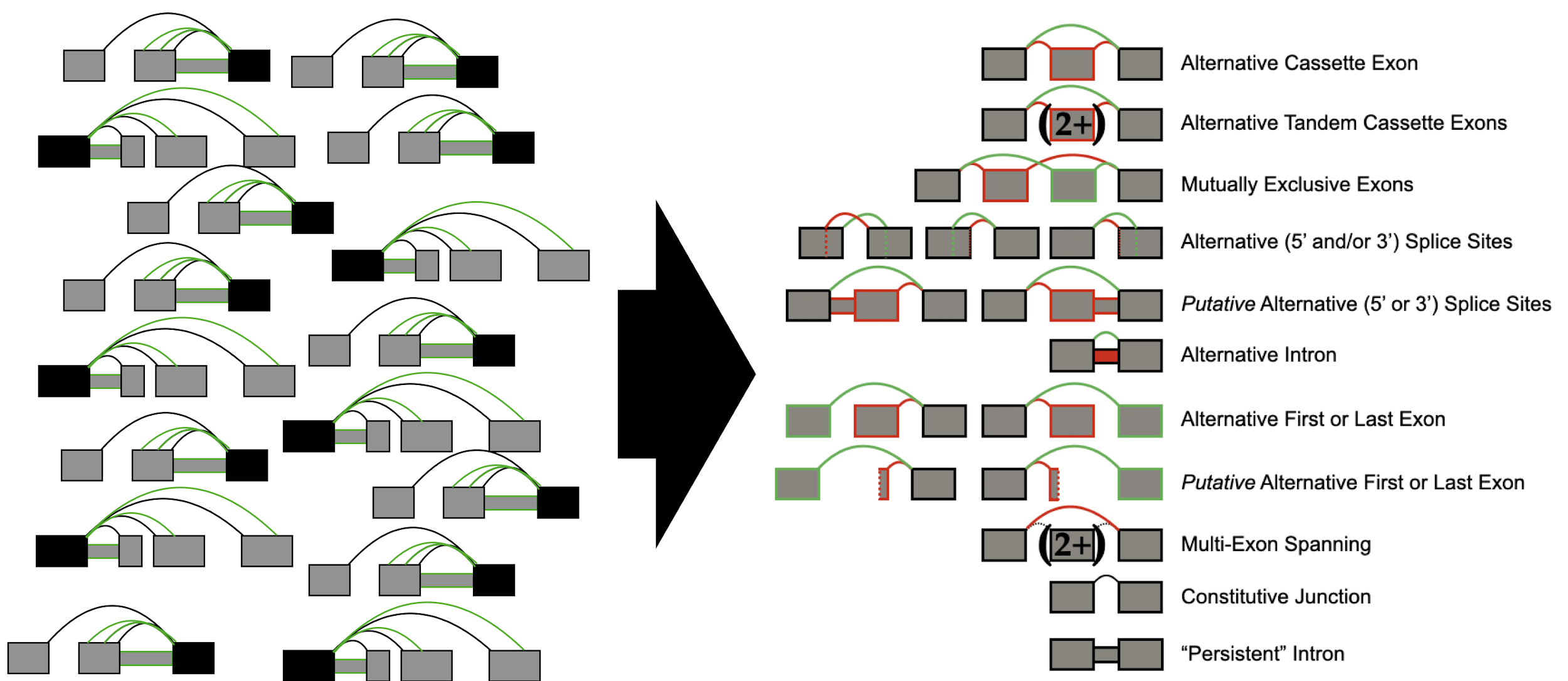
Categorizing splicing events with voila modulizer
We can also generate summaries of categorizations of splicing events with voila modulize. The purpose of this tool is not only to summarize classical events, but also a variety of complex events as well as determine common combinations of two or more events.
You may run the modulizer in the following manner:
[18]:
%%bash
voila modulize output/build/splicegraph.sql output/heterogen/*.het.voila -d output/modulized --overwrite
2023-10-11 12:46:08,649 (PID:44628) - INFO - Command: /home/sjewell/PycharmProjects/majiq/env_3.10/bin/voila modulize output/build/splicegraph.sql output/heterogen/HepG2_SRSF4KD-HepG2_NT.het.voila output/heterogen/HepG2_SRSF4KD-K562_NT.het.voila output/heterogen/K562_NT-HepG2_NT.het.voila output/heterogen/K562_SRSF4KD-HepG2_NT.het.voila output/heterogen/K562_SRSF4KD-HepG2_SRSF4KD.het.voila output/heterogen/K562_SRSF4KD-K562_NT.het.voila -d output/modulized --overwrite
2023-10-11 12:46:08,649 (PID:44628) - INFO - Voila v2.42.dev285+gcfe719c7.d20231011
2023-10-11 12:46:08,649 (PID:44628) - INFO - config file: /tmp/tmp68pqwnnk
2023-10-11 12:46:08,664 (PID:44628) - INFO - HETx6 MODULIZE
2023-10-11 12:46:08,672 (PID:44628) - INFO - Modulizing 8 gene(s)
2023-10-11 12:46:08,672 (PID:44628) - INFO - Quantifications based on 6 input file(s)
2023-10-11 12:46:08,672 (PID:44628) - INFO - ╔═══════════════════════════════════════════════════════════════╗
2023-10-11 12:46:08,672 (PID:44628) - INFO - ╠╡ Before Modulization:                                         ║
2023-10-11 12:46:08,672 (PID:44628) - INFO - ║     Dropping junctions with max(PSI) < 0.050                  ║
2023-10-11 12:46:08,672 (PID:44628) - INFO - ║     Dropping junctions with max(number_of_reads) < 1          ║
2023-10-11 12:46:08,672 (PID:44628) - INFO - ╠╡ After Modulization:                                          ║
2023-10-11 12:46:08,672 (PID:44628) - INFO - ║     Dropping modules if none(max(E(|dPSI|)) >= 0.200)         ║
2023-10-11 12:46:08,672 (PID:44628) - INFO - ║     Dropping modules if none(max(P(|dPSI|>=0.200)) >= 0.950)  ║
2023-10-11 12:46:08,672 (PID:44628) - INFO - ╚═══════════════════════════════════════════════════════════════╝
2023-10-11 12:46:08,673 (PID:44628) - INFO - Writing TSVs to /tmp/tmpucqll51w/output/modulized
2023-10-11 12:46:12,725 (PID:44628) - INFO - Concatenating Results
2023-10-11 12:46:12,810 (PID:44628) - INFO - Modulization Complete
Note that the modulizer can run with any combination of the standard .psi.voila or .deltapsi.voila files in addition to our het.voila files. Each additional piece of data for the same LSV/junction will be recorded in the output row in the modulized output.
The modulized output will be recorded in a number of files in .tsv format.
[19]:
ls output/modulized
alt3and5prime.tsv         heatmap.tsv              p_alt5prime.tsv
alt3prime.tsv             junctions.tsv            p_alternate_first_exon.tsv
alt5prime.tsv             multi_exon_spanning.tsv  p_alternate_last_exon.tsv
alternate_first_exon.tsv  mutually_exclusive.tsv   summary.tsv
alternate_last_exon.tsv   orphan_junction.tsv      tandem_cassette.tsv
alternative_intron.tsv    other.tsv
cassette.tsv              p_alt3prime.tsv
They are:
summary.tsv: Likely the most immediately useful for the majority of users. Each row corresponds to a splicing module, and lists the counts of each type of splicing event found inside the module.heatmap.tsv: For each module, a junction of greatest biological importance is considered and quantified here, one row per module. The method/parameters for choosing which junction is selected can be changed, seevoila modulize --helpfor details.event tsv files, ex:
cassette.tsv: Contains quantification information across all input files for each junction making up that specific splicing event.other.tsv: for any junctions not assigned to ANY splicing event, they are dumped here.junctions.tsv: A concatenation of all junction data from all event tsv files as well asother.tsv.
Please see VOILA modulizer documentation for more details on the modulizer.
Interactively visualizing results with voila view
We can also view results interactively in our web browser using voila view. We can start the web service by running
voila view output/build/splicegraph.sql output/heterogen/*.het.voila
By default, the web service is hosted on a random port for localhost (--host and -p flags can be used to specify directly). The console will print a URL that can be accessed from the same machine within a web browser. For example, when we run the above command, we see:
2021-09-01 01:08:53,380 (PID:5613) - INFO - Command: /{redacted}/bin/voila view output/build/splicegraph.sql output/heterogen/HepG2_SRSF4KD-HepG2_NT.het.voila output/heterogen/HepG2_SRSF4KD-K562_NT.het.voila output/heterogen/K562_NT-HepG2_NT.het.voila output/heteroge
n/K562_SRSF4KD-HepG2_NT.het.voila output/heterogen/K562_SRSF4KD-HepG2_SRSF4KD.het.voila output/heterogen/K562_SRSF4KD-K562_NT.het.voila
2021-09-01 01:08:53,380 (PID:5613) - INFO - Voila v2.2.0
2021-09-01 01:08:53,380 (PID:5613) - INFO - config file: /tmp/tmpixnu75yk
2021-09-01 01:08:53,395 (PID:5613) - INFO - Creating index: /{redacted}/output/heterogen/HepG2_SRSF4KD-HepG2_NT.het.voila
Indexing LSV IDs: 0 / 94
2021-09-01 01:08:55,510 (PID:5613) - INFO - Writing index: /{redacted}/output/heterogen/HepG2_SRSF4KD-HepG2_NT.het.voila
Serving on http://localhost:45899
So we open up http://localhost:45899 in our web browser. VOILA view first opens up to an index over genes/LSVs:
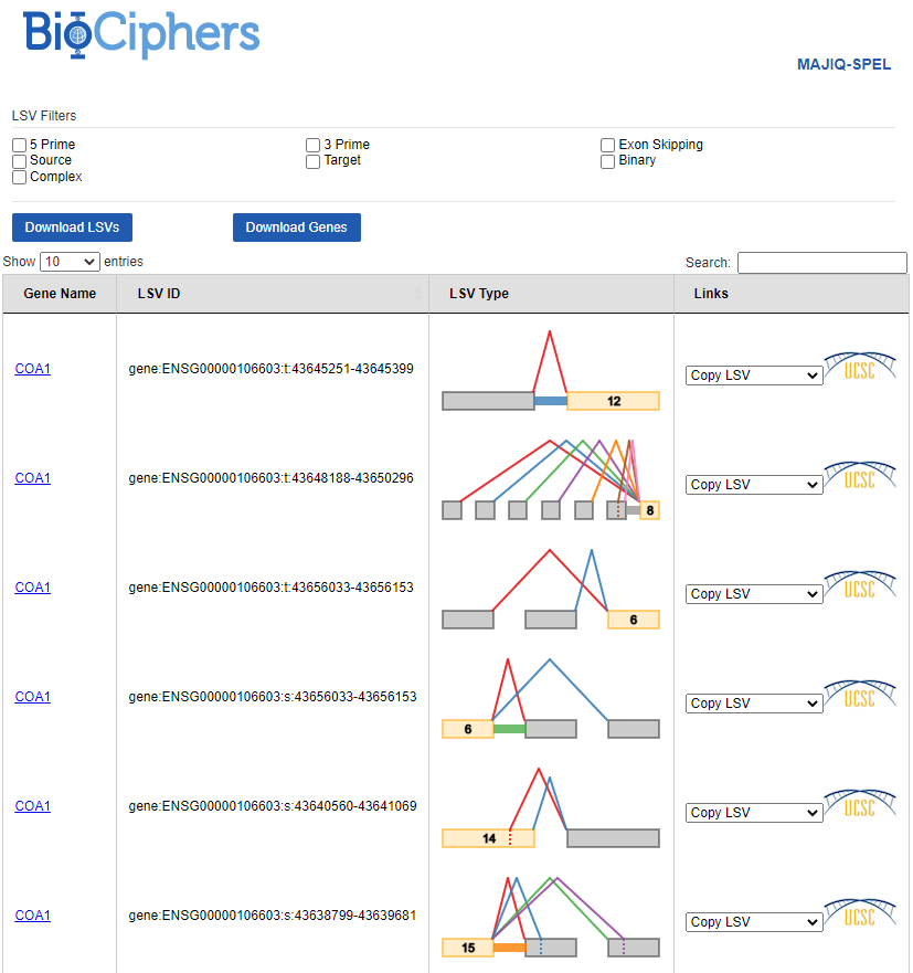
We can browse through pages of genes/LSV diagrams as convenient, or we can also use the search bar in the top-right hand side to search for a particular gene (or LSV). Once we’ve found a gene of interest, we click the link in the “Gene Name” column to view details for that gene.
For example, clicking into NDUFV3 gives us a screen that looks like:
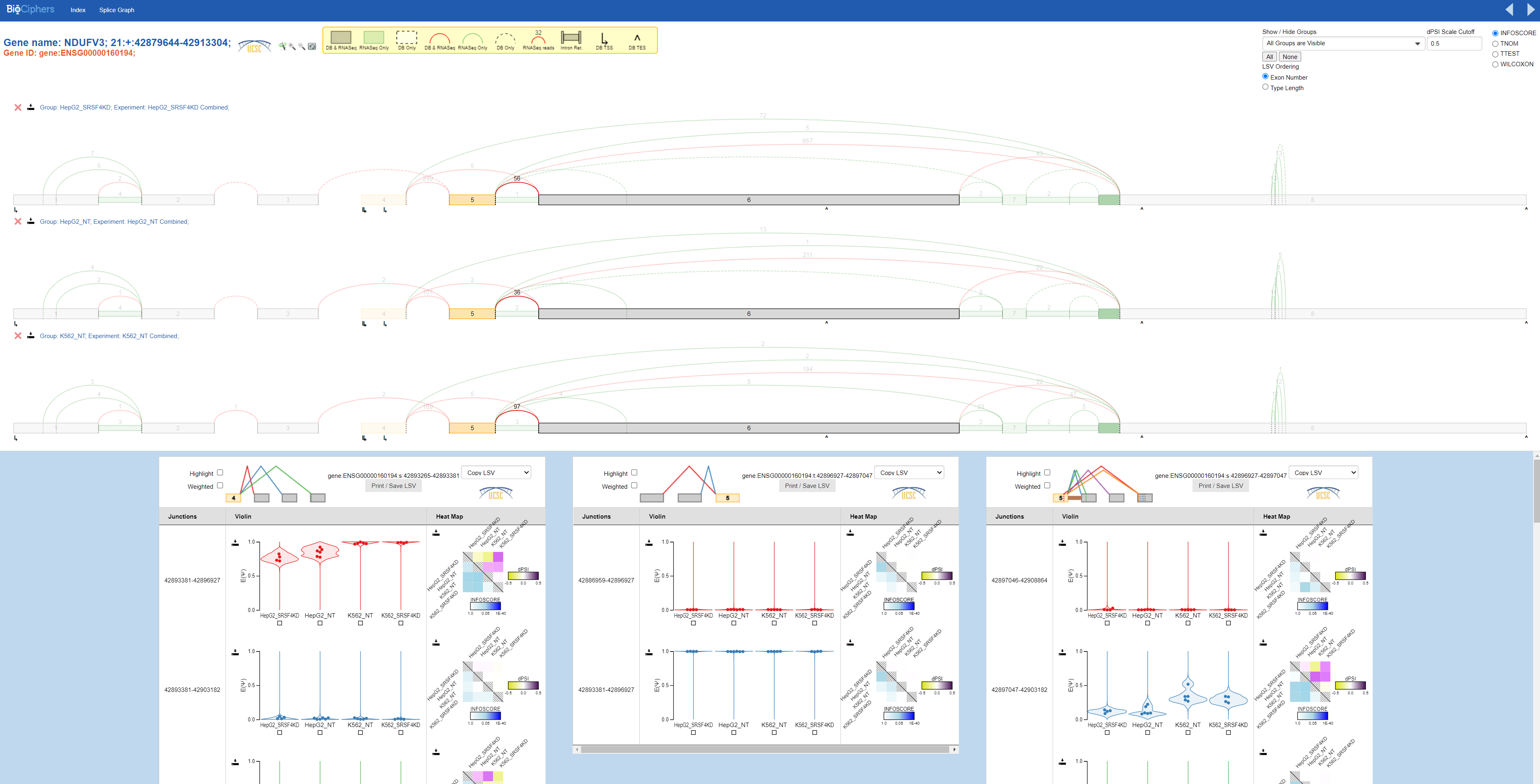
The top portion of the screen corresponds to splicegraphs. These indicate exon numbers and annotated vs denovo exons, junctions, and retained introns, and observed raw read coverage for each intron or junction. Which experiments have coverage displayed can be modified by clicking on the “SpliceGraph” button, and adding or removing additional experiments to display. The magnification buttons next to the legend allow zooming in or out on the splicegraph, and the wand button changes whether intronic regions are squashed or displayed to scale.
The bottom portion of the screen corresponds to quantified LSVs. Each LSV has three columns:
The first column indicates the genomic coordinates of the junction or retained intron.
The second column shows violin plots of the averaged posterior distributions per group. Individual points show the posterior means for PSI for each experiment per group. Hovering over points displays a tooltip indicating the experiment name.
The third column shows a heat map showing group-vs-group comparisons. Below the diagonal, the heatmap displays observed p-values for each comparison. The specific test displayed can be changed using the radio buttons in the top-right corner. Above the diagonal, the heatmap shows the difference in PSI between the medians of each group.
We can see the quantified values of PSI for each experiment per group in the violin plots.
voila view as a multi-user web server
voila view was also designed with sharing and collaboration in mind. So, in addition to being used locally, it is possible to set it up as its own web server host.
Note that accessibility of the service within local networks or the internet in general can be highly dependent on network settings and security practices (e.g. port forwarding, IP {white,black}lists, etc.) outside the scope of MAJIQ/VOILA itself; You can consult with your system administrator for advice if you want to make voila view available outside of the local machine / for multiple users.
voila viewhas a--hostparameter, which works similarly to--hostparameters in most other unix-like programs. That is, it sets the bind address. For the most common use case, to listen to all addresses, simply pass--host 0.0.0.0. (The default is--host 127.0.0.1, which listens only to your local machine)for security against port-scanners,
voila viewprovides a--enable-passcodeswitch. This generates a unique passcode in the link which is needed for users to successfully view the output. Recommended for use when hosting sensitive data with the tool.voila viewhas three web server options to cover all needs. you can chooseflask,waitress, orgunicornfor as a parameter to the--web-serverswitch.flaskis insecure and slow, and should only be used if you are trying to resolve a bizarre error, as it generates more debugging information.waitressis the default. It is efficient, and suitable for most single-user use cases. However, it is single-threaded.gunicornis a production-ready, performant web server used by many projects. It can serve many users/page requests concurrently. It may be helpful in some cases to speed up access even for a single user if loading very large numbers of LSVs in a gene at once. You can set the number of threads to host with the--num-web-workersargument. Safe to use with nginx proxy-pass as well.
Filtering results
The output files used by VOILA (splicegraph.sql, *.voila) can be very large for real analyses. voila filter allows filtering these files to reduce their filesize to facilitate sharing (or downloading from a cluster environment).
We:
specify the splicegraph
output/build/splicegraph.sqland voila filesoutput/heterogen/*.het.voilaas positional arguments,specify the output directory for the filtered files with the required argument
--directory output/voila_filterspecify the set of genes or LSVs to keep after filtering either directly (
--gene-ids,--lsv-ids) or by specifying a file with IDs to keep (--gene-ids-file,--lsv-ids-file):--gene-ids 'gene:ENSG00000106603'.
This leads to the command:
[20]:
%%bash
voila filter output/build/splicegraph.sql output/heterogen/*.het.voila \
    --directory output/voila_filter --gene-ids 'gene:ENSG00000106603' --overwrite
2023-10-11 12:46:13,977 (PID:44710) - INFO - Command: /home/sjewell/PycharmProjects/majiq/env_3.10/bin/voila filter output/build/splicegraph.sql output/heterogen/HepG2_SRSF4KD-HepG2_NT.het.voila output/heterogen/HepG2_SRSF4KD-K562_NT.het.voila output/heterogen/K562_NT-HepG2_NT.het.voila output/heterogen/K562_SRSF4KD-HepG2_NT.het.voila output/heterogen/K562_SRSF4KD-HepG2_SRSF4KD.het.voila output/heterogen/K562_SRSF4KD-K562_NT.het.voila --directory output/voila_filter --gene-ids gene:ENSG00000106603 --overwrite
2023-10-11 12:46:13,977 (PID:44710) - INFO - Voila v2.42.dev285+gcfe719c7.d20231011
2023-10-11 12:46:13,977 (PID:44710) - INFO - config file: /tmp/tmpmrp3ep9r
2023-10-11 12:46:13,989 (PID:44710) - INFO - HETx6 FILTER
2023-10-11 12:46:13,989 (PID:44710) - INFO - Filtering input to 1 gene(s)
2023-10-11 12:46:13,989 (PID:44710) - INFO - One splicegraph and 6 voila files
2023-10-11 12:46:13,989 (PID:44710) - INFO - Writing output files to /tmp/tmpucqll51w/output/voila_filter
2023-10-11 12:46:14,023 (PID:44740) - INFO - Started Filtering /tmp/tmpucqll51w/output/heterogen/HepG2_SRSF4KD-HepG2_NT.het.voila
2023-10-11 12:46:14,024 (PID:44742) - INFO - Started Filtering /tmp/tmpucqll51w/output/heterogen/HepG2_SRSF4KD-K562_NT.het.voila
2023-10-11 12:46:14,024 (PID:44744) - INFO - Started Filtering /tmp/tmpucqll51w/output/heterogen/K562_NT-HepG2_NT.het.voila
2023-10-11 12:46:14,024 (PID:44746) - INFO - Started Filtering /tmp/tmpucqll51w/output/heterogen/K562_SRSF4KD-HepG2_NT.het.voila
2023-10-11 12:46:14,025 (PID:44750) - INFO - Started Filtering /tmp/tmpucqll51w/output/heterogen/K562_SRSF4KD-K562_NT.het.voila
2023-10-11 12:46:14,024 (PID:44748) - INFO - Started Filtering /tmp/tmpucqll51w/output/heterogen/K562_SRSF4KD-HepG2_SRSF4KD.het.voila
2023-10-11 12:46:14,031 (PID:44744) - INFO - Finished writing output/voila_filter/K562_NT-HepG2_NT.het.voila
2023-10-11 12:46:14,032 (PID:44746) - INFO - Finished writing output/voila_filter/K562_SRSF4KD-HepG2_NT.het.voila
2023-10-11 12:46:14,032 (PID:44742) - INFO - Finished writing output/voila_filter/HepG2_SRSF4KD-K562_NT.het.voila
2023-10-11 12:46:14,033 (PID:44740) - INFO - Finished writing output/voila_filter/HepG2_SRSF4KD-HepG2_NT.het.voila
2023-10-11 12:46:14,033 (PID:44750) - INFO - Finished writing output/voila_filter/K562_SRSF4KD-K562_NT.het.voila
2023-10-11 12:46:14,034 (PID:44748) - INFO - Finished writing output/voila_filter/K562_SRSF4KD-HepG2_SRSF4KD.het.voila
2023-10-11 12:46:15,027 (PID:44744) - INFO - Filtering Splicegraph
2023-10-11 12:46:15,197 (PID:44744) - INFO - Finished Filtering Splicegraph
2023-10-11 12:46:16,030 (PID:44710) - INFO - Filtering Complete